Points and Coordinates

This section introduces the fundamental geometric entities of points and vectors, their mathematical representations, and coordinate systems used in linear algebra.

Euclidean Space and Coordinate Systems

The Cartesian Plane

This idea of relating the set of all points on a line to the real numbers goes back to antiquity, but it was not until the 17th century that mathematicians (notably Descartes and Fermat) developed a clear notion of how to coordinatize a plane: draw two perpendicular coordinatized lines (usually with the same scale on each) that intersect at their common origin. These lines are called the x-axis and y-axis. You can now uniquely identify every point on the plane using an ordered pair of numbers. If the point $P$ corresponds to the ordered pair $(x, y)$, then $x$ and $y$ are the coordinates of $P$.

The Number Line and Coordinates

Let's start with the one-dimensional case of a number line, a line labeled with real numbers. Select a point on the line to be the origin, denoted as $O$, and choose a direction to be positive. The positive direction is typically to the right, while the negative direction is to the left.

Suppose $p$ is a point on the number line that is located $x$ units to the right of the origin $O$. Then $x$ is called the coordinate of $p$, and $p$ is called the graph of $x$.

Suppose $q$ is a point on the number line that is located $x$ units to the left of $O$. Its distance from $O$ is still $x$, but it's not the same point as $p$. In this case, $-x$ is the coordinate of $q$, and $q$ is the graph of $-x$.

Points in 2D Euclidean Space

Now let's extend this idea to two dimensions (2D). We define a 2D coordinate system by drawing two perpendicular number lines that intersect at their common origin. The horizontal line is called the x-axis or the $\mathbf{e}_1$-axis, and the vertical line is called the y-axis or the $\mathbf{e}_2$-axis. Each axis has its own origin (the same point) and positive direction (right for x-axis, up for y-axis). By Euclid's definition of a plane, these two axes define a 2D Euclidean space, denoted as $\mathbb{E}^2$.

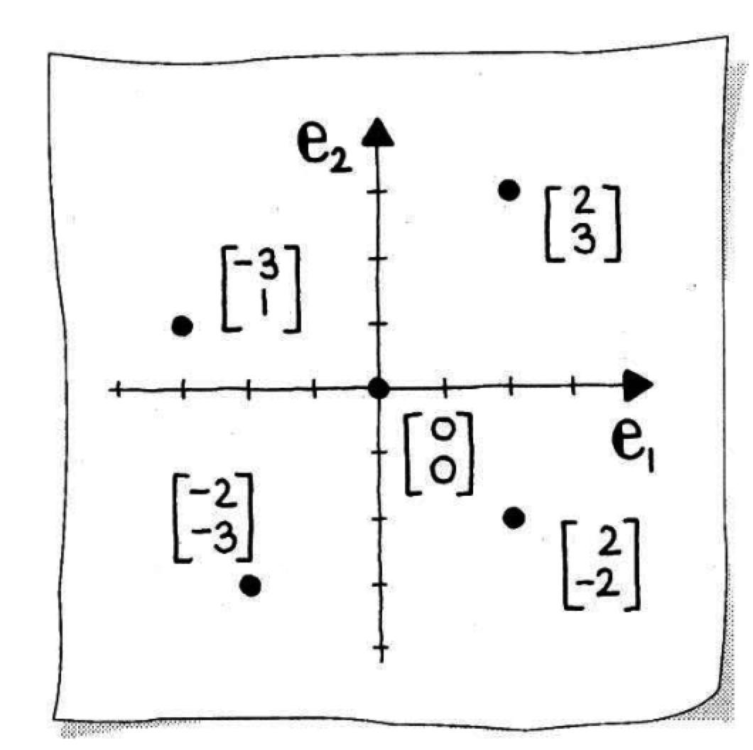
The most basic geometric entity is the point. A point $\mathbf{p}$ in 2D Euclidean space $\mathbb{E}^2$ is a reference to a location and can be represented by an ordered pair of coordinates $(p_1, p_2)$, where:

• \[p_1\]

  is the coordinate along the x-axis (horizontal direction)

• \[p_2\]

  is the coordinate along the y-axis (vertical direction)

The location of $\mathbf{p}$ is $p_1$-units along the $\mathbf{e}_1$-axis and $p_2$-units along the $\mathbf{e}_2$-axis. A point's coordinates, $p_1$ and $p_2$, are dependent upon the location of the coordinate origin, denoted as:

\[\mathbf{o}=\left\lbrack\begin{array}{l} 0 \\ 0 \end{array}\right\rbrack\]

We use boldface notation so there is a noticeable difference between a one-dimensional (1D) number, or scalar $p$, and a point $\mathbf{p}$.

To clearly identify $\mathbf{p}$ as a point, the notation $\mathbf{p} \in \mathbb{E}^2$ is used. This means that a 2D point "lives" in 2D Euclidean space $\mathbb{E}^2$.

Vectors

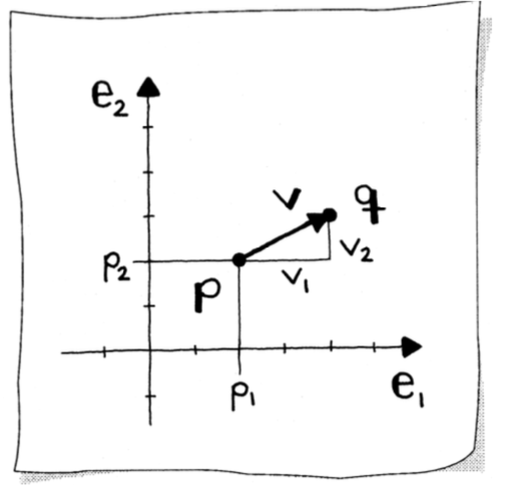
Suppose the reference point is $\mathbf{p}$, and when moving along a straight path, our target point is $\mathbf{q}$. The direction from $\mathbf{p}$ would be to follow the vector $\mathbf{v}$. Our notation for a vector is the same as for a point: boldface lowercase letters.

For algebraic properties of vector operations (addition, scalar multiplication, dot product), see Vector Operations in the Vectors document.

To get to $\mathbf{q}$ we say:

\[\mathbf{q}=\mathbf{p}+\mathbf{v}\]

To calculate this, add each component separately:

\[\left\lbrack\begin{array}{l} q_1 \\ q_2 \end{array}\right\rbrack=\left\lbrack\begin{array}{l} p_1 \\ p_2 \end{array}\right\rbrack+\left\lbrack\begin{array}{l} v_1 \\ v_2 \end{array}\right\rbrack=\left\lbrack\begin{array}{l} p_1+v_1 \\ p_2+v_2 \end{array}\right\rbrack\]

For example:

\[\left\lbrack\begin{array}{l} 4 \\ 3 \end{array}\right\rbrack=\left\lbrack\begin{array}{l} 2 \\ 2 \end{array}\right\rbrack+\left\lbrack\begin{array}{l} 2 \\ 1 \end{array}\right\rbrack\]

Vectors as Displacement

The components of $\mathbf{v}$, namely $v_1$ and $v_2$, indicate how many units to move along the $\mathbf{e}_1$- and $\mathbf{e}_2$-axis, respectively. This means that $\mathbf{v}$ can be defined as:

\[\mathbf{v}=\mathbf{q}-\mathbf{p}\]

This defines a vector as a difference of two points which describes a direction and a distance, or a displacement. The vector $\overrightarrow{PQ} = \mathbf{q} - \mathbf{p}$ is called the displacement vector from $\mathbf{p}$ to $\mathbf{q}$.

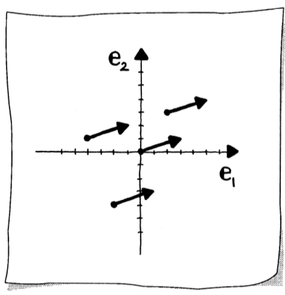
A vector has a tail and a head. The tail is typically displayed positioned at a point, or bound to a point, to indicate the geometric significance of the vector. However, unlike a point, a vector does not define a position. Two vectors are equal if they have the same component values, just as points are equal if they have the same coordinate values. Thus, considering a vector as a difference of two points, there are any number of vectors with the same direction and length.

Position Vectors and Free Vectors

A position vector is a vector from the origin $\mathbf{o}$ to a point $\mathbf{p}$:

\[\overrightarrow{OP} = \mathbf{p} - \mathbf{o} = \mathbf{p}\]

Since the origin has coordinates $\lbrack 0, 0 \rbrack$, the position vector of a point equals the point's coordinates.

A free vector is defined only by its magnitude and direction, not its starting point. As shown above, any number of vectors can have the same direction and length—these are all equal as free vectors. When we write $\mathbf{v} = \lbrack v_1, v_2 \rbrack$, we typically mean a free vector.

Special Vectors

A special vector worth mentioning is the zero vector:

\[\mathbf{0}=\left\lbrack\begin{array}{l} 0 \\ 0 \end{array}\right\rbrack\]

This vector has no direction or length.

Parallel Vectors

Two vectors are parallel if one is a scalar multiple of the other: $\mathbf{u} = c\mathbf{v}$ for some scalar $c$.

Linear Independence

Two vectors $\mathbf{v}$ and $\mathbf{w}$ describe a parallelogram (see parallelogram rule below). When this parallelogram has zero area, the two vectors are parallel—they satisfy $\mathbf{v} = c\mathbf{w}$ for some scalar $c$. In this case, we call them linearly dependent. Otherwise, they are linearly independent.

• Two vectors in $\mathbb{R}^2$ are linearly independent if they are not parallel (form a parallelogram with non-zero area)
• Two linearly independent vectors can express any other vector as a linear combination
• Two linearly independent vectors in 2D form a basis for $\mathbb{R}^2$

Example of linear dependence: The vectors $\mathbf{v} = \lbrack 1, 2 \rbrack$ and $\mathbf{w} = \lbrack 2, 4 \rbrack$ are linearly dependent since $\mathbf{w} = 2\mathbf{v}$. They lie on the same line through the origin and cannot span $\mathbb{R}^2$—for instance, $\mathbf{u} = \lbrack 1, 0 \rbrack$ cannot be written as $r\mathbf{v} + s\mathbf{w}$.

For the algebraic definition and properties of linear independence, see Linear Independence.

Span (Geometric View)

The span of a set of vectors is the set of all possible linear combinations of those vectors. Geometrically, the span represents all the points that can be "reached" by scaling and adding the vectors together.

Examples in $\mathbb{R}^2$:

• The span of one non-zero vector is a line through the origin in the direction of that vector
• The span of two non-parallel vectors is the entire plane $\mathbb{R}^2$
• The span of two parallel vectors (linearly dependent) is still just a line—the second vector adds no new directions

Connection to linear independence: Two vectors span $\mathbb{R}^2$ if and only if they are linearly independent. This is equivalent to saying their parallelogram has non-zero area.

For the algebraic definition of span, see Linear Combinations in the Vectors document.

Standard Basis

Other important vectors include the standard basis vectors:

\[\mathbf{e}_1=\left\lbrack\begin{array}{l} 1 \\ 0 \end{array}\right\rbrack \quad \text{and} \quad \mathbf{e}_2=\left\lbrack\begin{array}{l} 0 \\ 1 \end{array}\right\rbrack\]

These two vectors form the basis of our 2D representations of points and vectors:

\[\mathbf{p}=\mathbf{o}+p_1 \mathbf{e}_1+p_2 \mathbf{e}_2 \quad \text{and} \quad \mathbf{v}=v_1 \mathbf{e}_1+v_2 \mathbf{e}_2\]

They are often referred to as the standard basis in 2D.

Vector Spaces

To clearly identify $\mathbf{v}$ as a vector, we write $\mathbf{v} \in \mathbb{R}^2$. This means that a 2D vector "lives" in a 2D linear space $\mathbb{R}^2$. Other names for $\mathbb{R}^2$ are real or vector spaces.

Points vs Vectors

When writing a point or a vector, we use boldface lowercase letters; when programming, we use the same data structure (e.g., arrays). This makes it appear that points and vectors can be treated in the same manner. Not so!

Points and vectors are different geometric entities. This is reiterated by saying they live in different spaces: $\mathbb{E}^2$ and $\mathbb{R}^2$. For convenience and clarity, elements of Euclidean and linear spaces are typically displayed together.

The primary reason for differentiating between points and vectors is to achieve geometric constructions which are coordinate independent.

In what follows, let's use $\mathbf{p}, \mathbf{q} \in \mathbb{E}^2$ and $\mathbf{v}, \mathbf{w} \in \mathbb{R}^2$.

Coordinate Independent Operations

• Subtracting a point from another ($\mathbf{p}-\mathbf{q}$) yields a vector

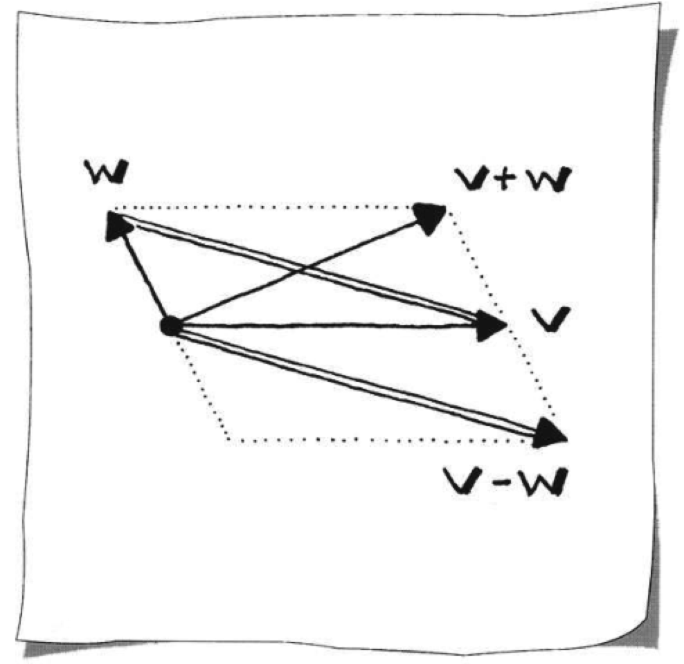
• Adding or subtracting two vectors yields another vector. The vectors $\mathbf{v}-\mathbf{w}$ and $\mathbf{v} + \mathbf{w}$ are the diagonals of the parallelogram defined by $\mathbf{v}$ and $\mathbf{w}$. This is a coordinate independent operation since vectors are defined as a difference of points (the parallelogram rule)

• Multiplying by a scalar $s$ is called scaling. Scaling a vector is a well-defined operation. The result $s\mathbf{v}$ adjusts the length by the scaling factor. The direction is unchanged if $s > 0$ and reversed for $s < 0$. If $s = 0$, then the result is the zero vector.

• Adding a vector to a point ($\mathbf{p}+\mathbf{v}$) yields another point.

Coordinate Dependent Operations

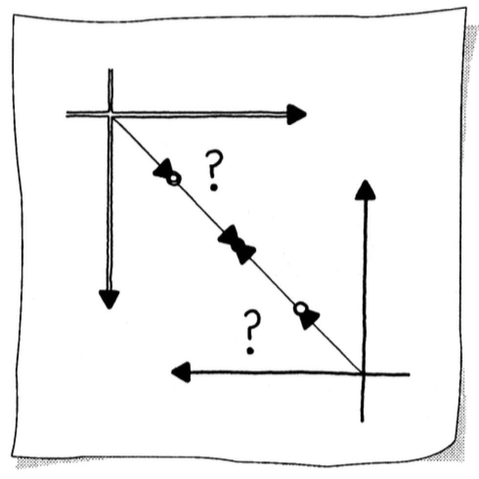
• Scaling a point ($s\mathbf{p}$) is not a well-defined operation. Scaling the solid black point by one-half with respect to two different coordinate systems results in two different points.

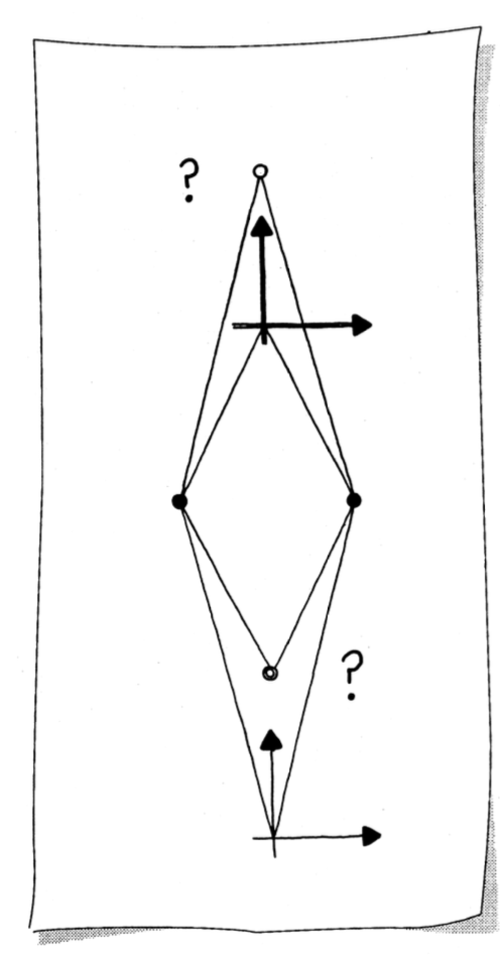
• Adding two points ($\mathbf{p}+\mathbf{q}$) is not a well-defined operation. The result of adding the two solid black points is dependent on the coordinate origin. (The parallelogram rule is used here to construct the results of the additions.)

Combining Points

Distance Between Points

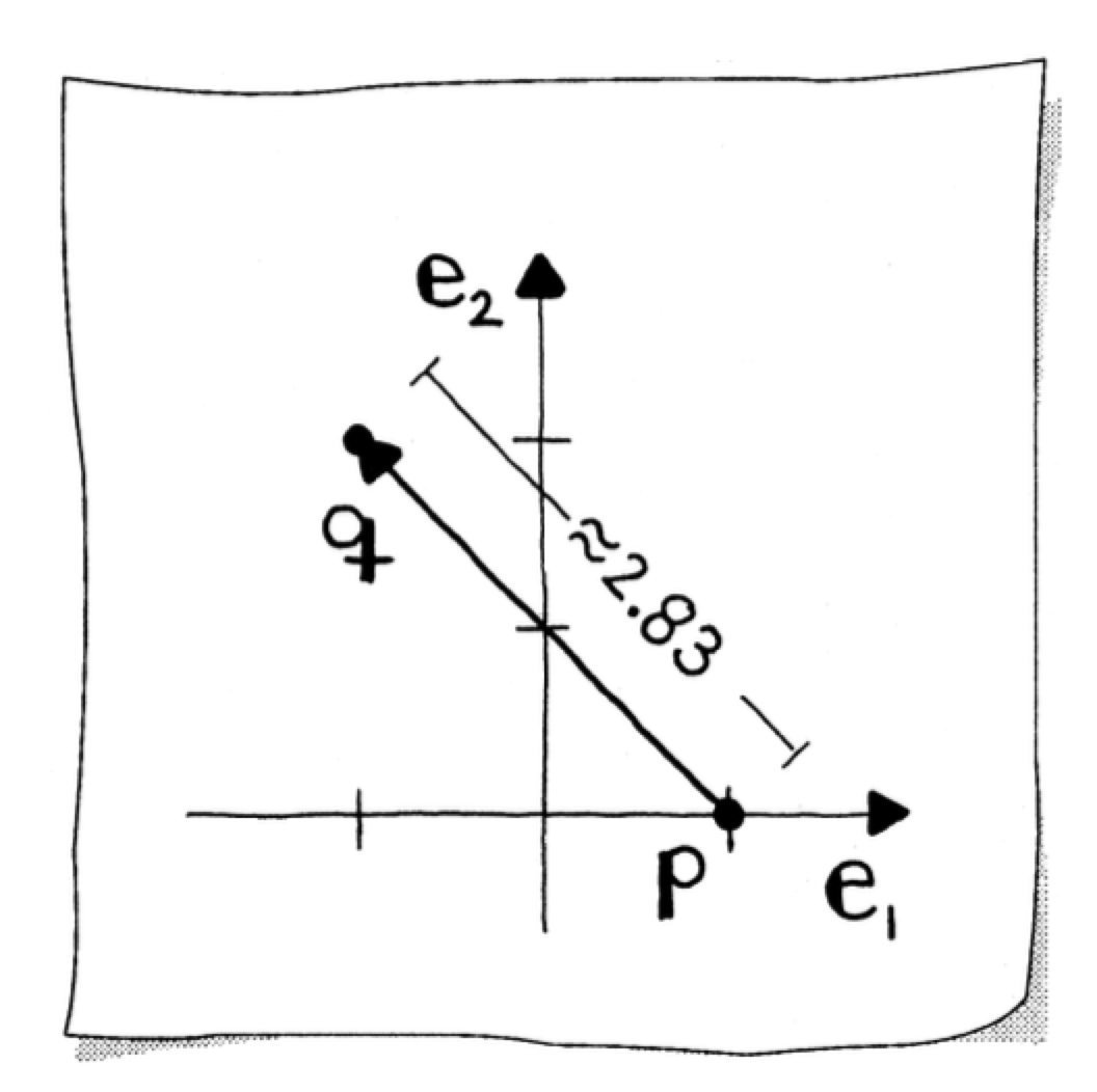
To find the distance between two points, we simply form a vector defined by the two points, e.g., $\mathbf{v}=\mathbf{q}-\mathbf{p}$, and apply the Euclidean norm:

\[\lVert\mathbf{v}\rVert=\sqrt{v_1^2+v_2^2}\]

Example: Let

\[\mathbf{q}=\left\lbrack\begin{array}{r} -1 \\ 2 \end{array}\right\rbrack \quad \text{and} \quad \mathbf{p}=\left\lbrack\begin{array}{l} 1 \\ 0 \end{array}\right\rbrack\]

Then

\[\mathbf{q}-\mathbf{p}=\left\lbrack\begin{array}{r}-2 \\ 2\end{array}\right\rbrack\]

and

\[\lVert\mathbf{q}-\mathbf{p}\rVert=\sqrt{(-2)^2+2^2}=\sqrt{8} \approx 2.83\]

using GeometryBasics
using LinearAlgebra

function distance_2_points(p::Point, q::Point)
    v = q - p
    norm(v)
end

julia> p = Point(1, 0)
julia> q = Point(-1, 2)
julia> distance_2_points(p, q)
2.8284271247461903

Midpoint of Two Points

There is a way to combine two points such that we get a meaningful third one. Take the example of the midpoint $\mathbf{r}$ of two points $\mathbf{p}$ and $\mathbf{q}$:

\[\mathbf{p}=\left\lbrack\begin{array}{l}1 \\ 6\end{array}\right\rbrack, \quad \mathbf{r}=\left\lbrack\begin{array}{l}2 \\ 3\end{array}\right\rbrack, \quad \mathbf{q}=\left\lbrack\begin{array}{l}3 \\ 0\end{array}\right\rbrack\]

Start with the known coordinate independent operation of adding a vector to a point. Define $\mathbf{r}$ by adding an appropriately scaled version of the vector $\mathbf{v}=\mathbf{q}-\mathbf{p}$ to the point $\mathbf{p}$:

\[\begin{aligned} \mathbf{r} & =\mathbf{p}+\frac{1}{2} \mathbf{v} \\ \left\lbrack\begin{array}{l} 2 \\ 3 \end{array}\right\rbrack & =\left\lbrack\begin{array}{l} 1 \\ 6 \end{array}\right\rbrack+\frac{1}{2}\left\lbrack\begin{array}{r} 2 \\ -6 \end{array}\right\rbrack \end{aligned}\]

Expanding, this shows that $\mathbf{r}$ can also be defined as:

\[\begin{aligned} \mathbf{r} & =\frac{1}{2} \mathbf{p}+\frac{1}{2} \mathbf{q} \\ \left\lbrack\begin{array}{l} 2 \\ 3 \end{array}\right\rbrack & =\frac{1}{2}\left\lbrack\begin{array}{l} 1 \\ 6 \end{array}\right\rbrack+\frac{1}{2}\left\lbrack\begin{array}{l} 3 \\ 0 \end{array}\right\rbrack \end{aligned}\]

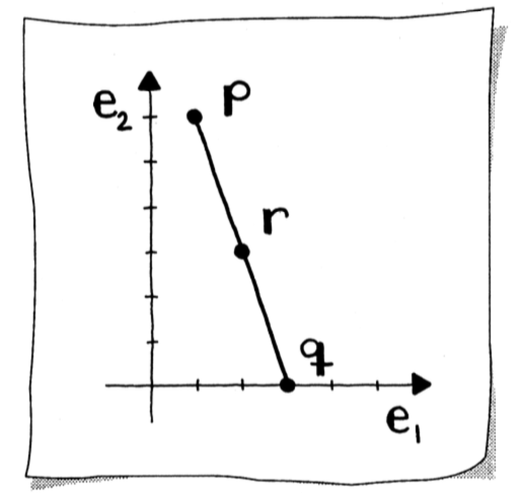
This is a legal expression for a combination of points.

Combining Points to Form Vectors

We can also combine points so that the result is a vector. For this, we need the coefficients to sum to zero. Suppose we have the equation:

\[\mathbf{e}=\mathbf{r}-2 \mathbf{p}+\mathbf{q}, \quad \mathbf{r}, \mathbf{p}, \mathbf{q} \in \mathbb{E}^2\]

Does $\mathbf{e}$ have a geometric meaning? Looking at the sum of the coefficients, $1-2+1=0$, we conclude that $\mathbf{e}$ is a vector. By rewriting the equation as:

\[\mathbf{e}=(\mathbf{r}-\mathbf{p})+(\mathbf{q}-\mathbf{p})\]

it is clear that $\mathbf{e}$ is a vector formed from (vector + vector).

Barycentric Coordinates

Adding a (scaled) vector to a point is a well-defined, coordinate independent operation that yields another point. Any point of the form:

\[\mathbf{r}=\mathbf{p}+t \mathbf{v}\]

is on the line through $\mathbf{p}$ and $\mathbf{q}$. We may rewrite this as:

\[\mathbf{r}=\mathbf{p}+t(\mathbf{q}-\mathbf{p})\]

and then:

\[\mathbf{r}=(1-t) \mathbf{p}+t \mathbf{q}\]

The scalar values $(1-t)$ and $t$ are coefficients. A weighted sum of points where the coefficients sum to one is called a barycentric combination. In this special case, where one point $\mathbf{r}$ is being expressed in terms of two others, $\mathbf{p}$ and $\mathbf{q}$, the coefficients $1-t$ and $t$ are called the barycentric coordinates of $\mathbf{r}$.

Linear Interpolation

A barycentric combination allows us to construct $\mathbf{r}$ anywhere on the line defined by $\mathbf{p}$ and $\mathbf{q}$. This is why $\mathbf{r}$ is also called linear interpolation.

• Convex combinations: To restrict $\mathbf{r}$'s position to the line segment between $\mathbf{p}$ and $\mathbf{q}$, we allow only values where $0 \leq t \leq 1$
• Extrapolation: To define points outside of the line segment between $\mathbf{p}$ and $\mathbf{q}$, we need values of $t<0$ or $t>1$

Ratio and Center of Gravity

The position of $\mathbf{r}$ is said to be in the ratio of $t:(1-t)$ or $t/(1-t)$. In physics, $\mathbf{r}$ is known as the center of gravity of two points $\mathbf{p}$ and $\mathbf{q}$ with weights $1-t$ and $t$, respectively.

From a constructive approach, the ratio is formed from the quotient:

\[\text{ratio}=\frac{\lVert\mathbf{r}-\mathbf{p}\rVert}{\lVert\mathbf{q}-\mathbf{r}\rVert}\]

Parameter Definition

The barycentric coordinate $t$ is also called a parameter. This parameter is defined by the quotient:

\[t=\frac{\lVert\mathbf{r}-\mathbf{p}\rVert}{\lVert\mathbf{q}-\mathbf{p}\rVert}\]

function center_of_gravity(p::Point, q::Point, t::Float64)
    v = q - p
    r = p + (t * v)
end

function barycentric_coord(p::Point, q::Point, r::Point)
    t = norm(r - p) / norm(q - r)
end

julia> p = Point(2, 2)
julia> q = Point(6, 4)
julia> r = center_of_gravity(p, q, 2.0)
Point2{Float64}(10.0, 6.0)

julia> barycentric_coord(p, q, r)
2.0

Barycentric Combinations with Three Points

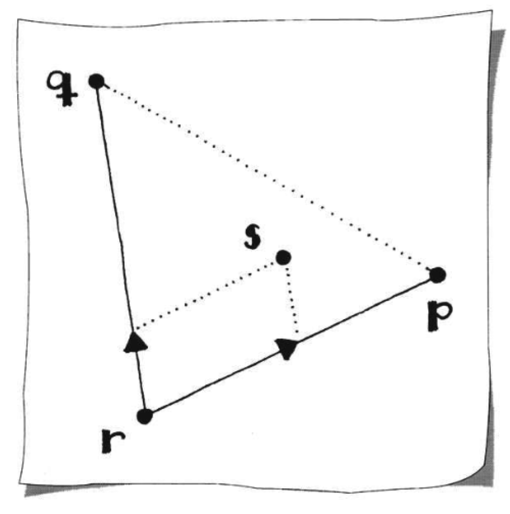
We can create barycentric combinations with more than two points. Consider three points $\mathbf{p}$, $\mathbf{q}$, and $\mathbf{r}$ which are not collinear. Any point $\mathbf{s}$ can be formed from:

\[\mathbf{s}=\mathbf{r}+t_1(\mathbf{p}-\mathbf{r})+t_2(\mathbf{q}-\mathbf{r})\]

This is a coordinate independent operation of point + vector + vector. Expanding and regrouping, we can also define $\mathbf{s}$ as:

\[\begin{aligned} \mathbf{s} & =t_1 \mathbf{p}+t_2 \mathbf{q}+\left(1-t_1-t_2\right) \mathbf{r} \\ & =t_1 \mathbf{p}+t_2 \mathbf{q}+t_3 \mathbf{r} \end{aligned}\]

Thus, the point $\mathbf{s}$ is defined by barycentric combination with coefficients $t_1$, $t_2$, and $t_3=1-t_1-t_2$ with respect to $\mathbf{p}$, $\mathbf{q}$, and $\mathbf{r}$, respectively.

Point-Tester Equations

Identifying $\mathbb{R}^2$ with a plane provides a way to use algebra to describe geometric objects. This is the central theme of analytic geometry.

Consider the circle $C$. You can describe $C$ geometrically by saying that $C$ consists of all points in the plane that are 1 unit from the origin $O$. However, you can also describe $C$ algebraically in terms of the coordinates of the points that lie on $C$: the circle $C$ is the set of points $(x, y)$ so that $x^2+y^2=1$.

The connection between the geometric description ("$C$ consists of all points...") and the equation ("$x^2+y^2=1$") is that the equation is a point-tester for the geometric definition. This means you can test a point to see if it's on the circle by checking if its coordinates satisfy the equation.

Example: Test if the point $\left(\frac{\sqrt{2}}{2}, \frac{\sqrt{2}}{2}\right)$ lies on the unit circle:

\[\left(\frac{\sqrt{2}}{2}\right)^2 + \left(\frac{\sqrt{2}}{2}\right)^2 = \frac{1}{2} + \frac{1}{2} = 1 \quad \checkmark\]

This approach generalizes to any geometric object: lines, ellipses, parabolas, and more complex curves can all be described by point-tester equations.